This is a guest post on my website. It is written by Johan Holwerda about the SDF editor he built for the RenderQueue.
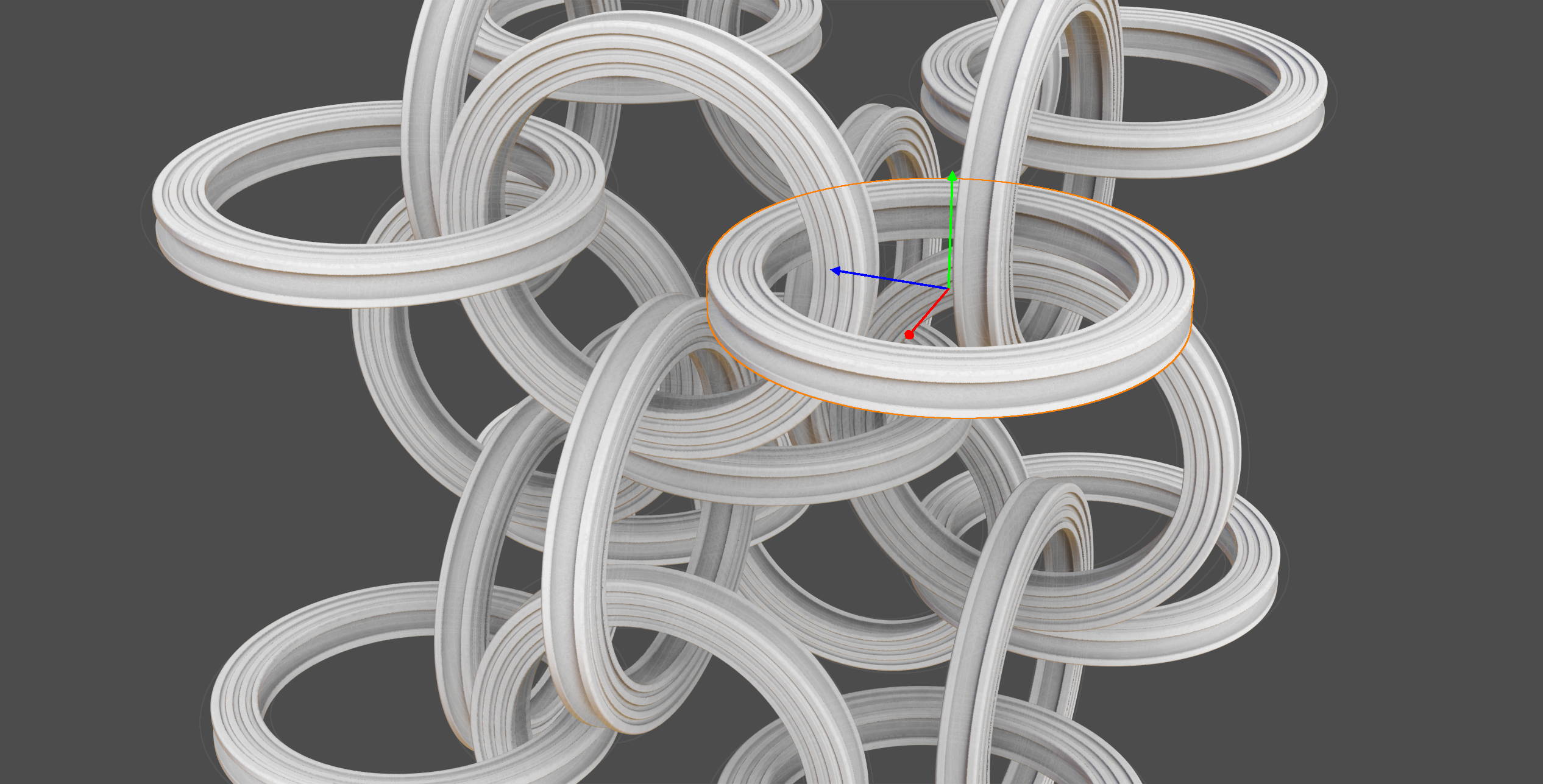
I’ve been working on a WebGPU-based SDF editor for modeling using signed distance field shapes. The editor supports hierarchical scene graphs with groups and primitives, with blend operations and blend radius for both. You can find the demo here.
In this post, I’ll go through the technical details of how the rendering pipeline works.
What Are Signed Distance Fields?
A signed distance field (SDF) is a function that, for any point in space, returns the distance to the nearest surface. The sign indicates whether the point is inside (negative) or outside (positive) the geometry. SDFs are powerful because they make certain operations trivial: smooth blending between shapes, boolean operations, and surface extraction all become straightforward mathematical operations.
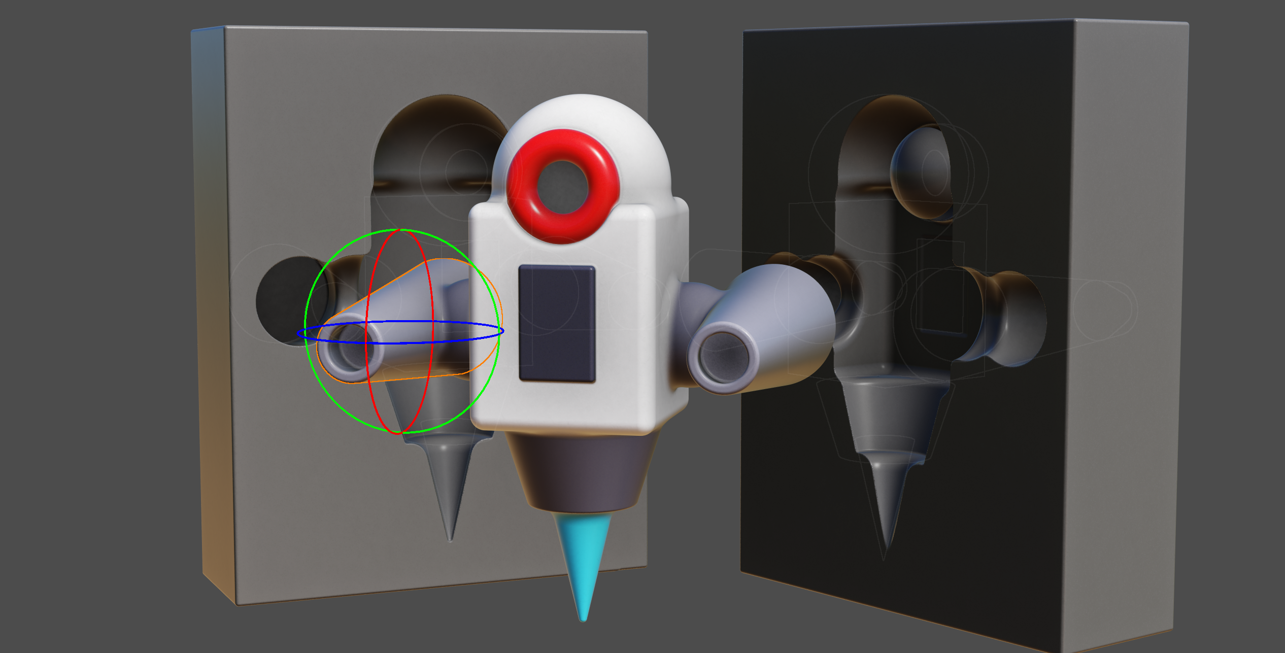
The editor supports six primitive shapes:
- Sphere – defined by a radius
- Box – defined by three half-extents
- Torus – defined by major and minor radii
- Capsule – a line segment with a radius
- Cylinder – defined by height and radius
- Cone – a cylinder with independent top and bottom radii
Each primitive can be combined using three blend operations: union (add), subtraction (carve out), and intersection (keep overlap). All operations support smooth blending with a configurable radius.
The Rendering Pipeline
The rendering pipeline consists of several stages, each running as GPU compute shaders. Here’s an overview of how a frame is rendered:
- Update primitive buffer with transforms and properties (on the CPU)
- Space partitioning – assign primitives to grid cells
- Dirty mask – detect which cells need re-evaluation
- Octree split – find cells that contain surfaces
- Surface extraction (Marching Cubes or Surface Nets)
- Ambient occlusion via shadow maps
- Final rendering with temporal anti-aliasing
Step 1: The Primitive Buffer
All scene data is stored in a single GPU buffer. Each primitive (or group) occupies 28 floats (112 bytes) containing:
struct Primitive {
    rotation: vec4<f32>,       // Inverse quaternion rotation
    positionScale: vec4<f32>,  // World position + uniform scale
    bbMinParent: vec4<f32>,    // Bounding box min + parent index
    bbMaxSubTree: vec4<f32>,   // Bounding box max + subtree size
    blendInfo: vec4<f32>,      // Blend type, radius, max blend radius, index
    colorShape: vec4<f32>,     // RGB color + shape type
    radii: vec4<f32>,          // Shape-specific dimensions + roundness
}
Code language: GLSL (glsl)
Unfortunately the vec4 packing was needed to make it work on chrome on android.
The scene is organized as a hierarchical tree where groups can contain other groups or primitives. On the CPU side, bounding boxes are computed recursively: primitives calculate their own bounds based on shape type and transform, while groups derive their bounds from their children.
The bounding box calculation takes blend operations into account. A subtraction or intersection can only shrink the parent’s bounds, so we can compute tighter AABBs for the entire hierarchy.
Step 2: Primitive Space Partitioning
Before we can evaluate the SDF efficiently, we need to know which primitives could potentially influence each region of space. The world is divided into a 3D grid (up to 2^14 = 16,384 cells), and each primitive is assigned to all cells its bounding box overlaps. This is done in a compute shader that:
- Iterates over all cells in parallel
- For each cell, checks which primitives could influence it (based on bounding box + blend radius overlap)
- Outputs a list of primitive indices per cell The primitive lists are then sorted by cell index using a counting sort algorithm.
The result is stored as a prefix sum buffer, allowing any shader to quickly look up which primitives affect a given cell. This spatial partitioning is important for performance as the hierarchy supports thousands of primitives.
How Counting Sort Works Here
The counting sort algorithm organizes primitive-to-cell assignments into a compact, GPU-friendly format. It works in three passes:
- Count: Each cell runs in parallel. For each primitive that influences the cell, use
atomicAddon a global counter to claim a slot. At that slot, store the primitive index, the cell index, and the index of this primitive within its cell (a simple per-thread counter). At the end, store the total count for this cell. - Prefix sum: Transform the per-cell counts into cumulative offsets. After this step,
prefixSum[cellIndex]tells us where that cell’s primitives end in the final sorted array. The prefix sum runs on 2^14 cells and is split into a 4-level tree structure so the longest loop is 16 iterations. - Scatter: Write each primitive to its final sorted position. Since we already know each primitive’s index within its cell, no atomics are needed here:
let cellIndex = keys[i];
var o = 0u;
if(cellIndex > 0){
	o = offsetPerTile[cellIndex - 1u];
}
sortedItems[o + indexWithinTile[i]] = items[i];
Code language: JavaScript (javascript)
Each primitive is touched once during the scatter pass. The result is a flat array of primitive indices sorted by cell, and any shader can look up the relevant primitives for a cell in constant time.
Step 3: Dirty Mask
When editing, most of the scene remains unchanged. The dirty mask system detects which cells have been modified since the last frame.
The shader compares the current primitive buffer with a cached copy from the previous frame. If any primitive affecting a cell has changed (position, rotation, shape parameters, etc.), that cell is marked as dirty.
During editing, only dirty cells need to be re-evaluated. Unchanged regions reuse their previous geometry, which makes interactive editing feel responsive even with complex scenes.
Step 4: Octree Split
Not every grid cell contains part of the surface. Before running surface extraction, we first identify which cells potentially contain geometry.
The octree fill pass uses a hierarchical approach:
- Start with the coarse grid (the “low resolution” cells from the dirty mask)
- For each low-res cell, check if any high-res sub-cells might contain a surface
- Output only the cells that need processing for the next iteration of octree split
A cell potentially contains a surface if the SDF value is lower than sqrt(3) * .5 * cellSize. Depending on the quality setting, the splitting happens 4 to 6 times. At the 6th split cell indices are 32 bit and we can’t go deeper without doubling the size of the cell index buffer.
Step 5: Surface Extraction
The editor supports two surface extraction algorithms, each with different trade-offs.
Marching Cubes (Edit Mode)
During interactive editing, speed is more important than quality. Marching Cubes generates triangles directly:
- Sample the SDF at the 8 corners of each cell
- Look up the triangulation pattern in a precomputed table (256 possible configurations)
- Interpolate vertex positions along cell edges based on SDF values
- Output packed triangles to a buffer
The triangles are packed into 16 bytes each: triangle position is stored as cell index and the vertex positions are relative to that, normal is derived from the vertices positions, and color is stored per-triangle. This way we can fit 32M triangles in a 512MB buffer.
A ping-pong buffer system preserves geometry from unchanged cells: when a cell is marked clean, its triangles are copied to the output buffer; only dirty cells generate new geometry.
Surface Nets (View Mode)
When the user stops editing, Surface Nets provides cleaner output with one vertex per cell rather than multiple triangles:
- For each cell containing a surface crossing, compute a single vertex position
- Position is determined by averaging the edge crossings within the cell
- Color is sampled from the SDF at the vertex position
Surface Nets gives vertices a more uniform distribution, which is better for the per-point ambient occlusion and point rendering. Vertices take 12 bytes each (position, normal, color).
Step 6: Ambient Occlusion
Once the geometry is made, the editor computes ambient occlusion with a shadow map approach:
- Generate 1024 camera positions uniformly distributed on a sphere (Fibonacci spiral)
- For each batch of 16 directions:
- Render the scene to a depth buffer from that direction
- For each vertex, check if it’s visible from that direction
- Accumulate occlusion values
The points are assigned to one of the 16 shadow camera projections and drawn in a single pass. Every point draws to only one shadow map. The shadow maps are rendered in compute shaders by writing depth with atomic max. Each vertex samples 16 shadow maps per frame and accumulates a visibility count. The final AO value is the ratio of visible samples to total samples. This approach spreads the AO computation over multiple frames.
I have tried ray-marching the distance function and a hybrid screenspace approach, but these experiments had a worse performance / quality trade-off.
Step 7: Final Rendering
The final render pass combines everything:
Point Rendering
In view mode, Surface Nets vertices are rendered as points. Each point is shaded using the accumulated AO value, surface normal (computed from the SDF gradient), and the primitive color. The points are sized to fill the screen without gaps.
Rendering with points is not perfect. When zooming in, individual points become visible and sharp edges look ‘blobby’. On most screens though, when viewing the complete model, a point ends up being about 1 pixel—which gives enough detail for the effect I was going for.
I considered rendering with triangles instead, but that turned out to be about 5 times slower for 1-pixel triangles, and uses more memory. The main difficulty is finding neighboring vertices to form triangles. With 2^32 cells in high quality mode, a lookup buffer would be 4 billion entries, which is too large. A hashmap would work but adds complexity and overhead. I tried a scheme with localized buffers distributed around the surface, which worked, but it limited the maximum vertex count more than I liked. I might revisit this later.
For depth testing, each vertex writes its depth using atomic max. If the write succeeds (depth changed), it also writes its vertex index to a screen buffer. This two-step approach is needed because WebGPU doesn’t support 64-bit atomics—otherwise depth and index could be packed together.
The downside is that when multiple points compete for the same pixel, the wrong vertex index can end up stored. The shading pass detects this by reprojecting the vertex and comparing depths. Mismatches are flagged as errors (output as 1,0,0,0) and the TAA pass rejects these pixels, falling back to the previous frame’s value instead
Temporal Anti-Aliasing
To reduce aliasing, fix errors, and fill small holes, the renderer uses temporal anti-aliasing (TAA). Each frame, the camera projection is jittered by a sub-pixel offset. The current frame is blended with the previous frames using an exponential moving average, this smooths out edges and averages sub-pixel points when the camera is stationary.
Evaluating the SDF
The core of the system is the distance evaluation function. Given a point in space, it must return the signed distance to the surface, correctly handling the hierarchical group structure and blend operations.
The algorithm uses a stack to track group state:
fn getDistance(p: vec3<f32>, cellIndex: u32, cellSize: f32) -> f32 {
    var groupStack: array<GroupStackEntry, MAX_GROUP_DEPTH>;
    var stackDepth = 0u;
    var currentDistance = dMax;

    for (var i = startIndex; i < endIndex; i++) {
        let prim = primitiveBuffer[primitiveIndexBuffer[i]];

        // Close groups that should end before this primitive
        while (stackDepth > 0u) {
            if (groupStack[stackDepth - 1].groupIndex > abs(prim.parentIndex)) {
                stackDepth -= 1u;
                currentDistance = blendDistances(
                    groupStack[stackDepth].blendType,
                    groupStack[stackDepth].distance,
                    currentDistance,
                    groupStack[stackDepth].blendRadius
                );
            } else {
                break;
            }
        }

        if (prim.hasChildren) {
            // Push group onto stack
            groupStack[stackDepth] = GroupStackEntry(
                prim.index, currentDistance, prim.blendType, prim.blendRadius
            );
            stackDepth += 1u;
            currentDistance = dMax;
        } else {
            // Evaluate primitive and blend
            let dist = getPrimitiveDistance(p, prim);
            currentDistance = blendDistances(
                prim.blendType, currentDistance, dist, prim.blendRadius
            );
        }
    }

    // Close remaining groups
    while (stackDepth > 0u) {
        // ... blend with parent distance
    }

    return currentDistance;
}
Code language: JavaScript (javascript)
The primitives are ordered depth-first in the buffer, so the stack naturally tracks the hierarchy as we iterate through the list.
Limitations
- Vertex buffer size: The 512 MB buffer fits about 44M points. Models with lots of surface area but little volume can exceed this quickly.
- Overdraw: Unlike raymarching, the point renderer may draw to the same pixel multiple times. Thin, detailed surfaces are more expensive to render.
- Moving large objects: Slow, because many cells need to be updated.
- Normal precision: Currently a bit low. Grouping points into batches with per-batch bounding boxes would allow better precision without increasing memory.
- UI: Could use some work.
TODO
- OBJ export: The marching cubes exporter works but produces huge files slowly. Exporting indexed surface net triangles would be much better.
- Gallery: A gallery of user creations would be nice.
- World space transforms: Translation and rotation in world space.
- Object locking: Prevent accidental edits.
- Multi-select: Select and manipulate multiple objects at once.
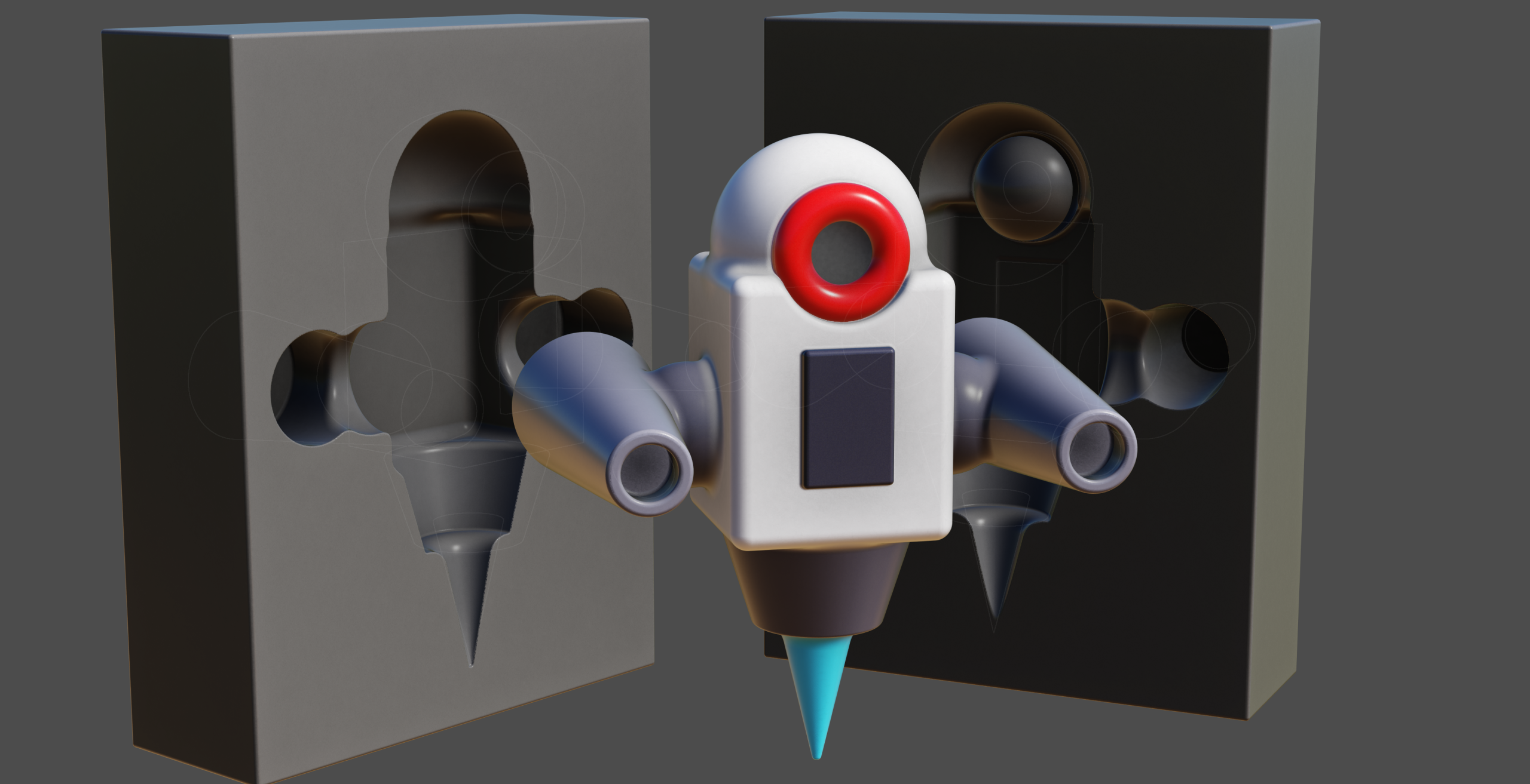
The RenderQueue
I have pushed this experiment to the RenderQueue. You can find it here.